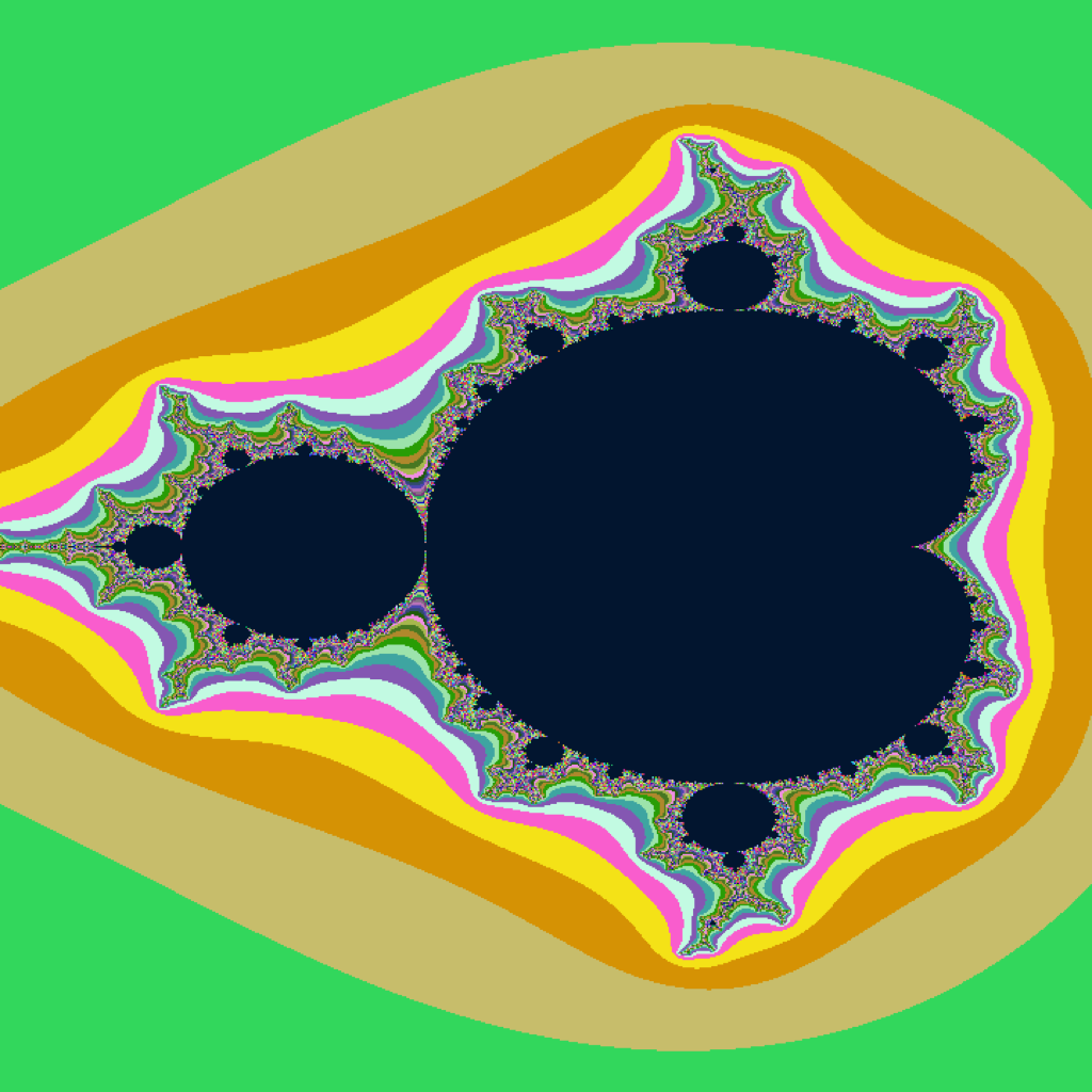
A technical companion for readers comfortable with a little calculus and complex numbers. Every formula and constant below is drawn directly from DoomFracting's own C and Swift source — where the app deliberately doesn't do something, that's noted rather than glossed over.
The Mandelbrot set, and Julia sets
Fix a complex number \(c = c_x + i c_y\). Iterate the map \(z_{n+1} = z_n^2 + c\), starting at \(z_0 = 0\). The Mandelbrot set \(M\) is the set of every \(c\) for which this orbit stays bounded forever:
A bailout radius stands in for "definitely escapes": DoomFracting uses 256 — comparing the squared modulus against 65,536 rather than taking a square root — a much larger margin than the mathematically-sufficient 2, chosen so the smooth coloring formula in Part II stays numerically well-behaved.
Julia sets: the same formula, roles reversed
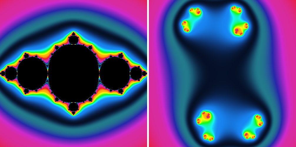
Now fix \(c\) and let \(z_0\) range over the whole plane instead. The same map defines the filled Julia set \(K_c\). Every point \(c\) has its own Julia set — DoomFracting's "swap to Julia" feature renders exactly the Julia set for whichever \(c\) your Mandelbrot view is centered on, full-screen.
Fatou–Julia dichotomy. A Julia set \(J_c\) is either connected (one piece), or totally disconnected "Fatou dust" — never in between. And \(J_c\) is connected if and only if \(c \in M\). This is why \(M\) is called the connectedness locus: a map of which Julia sets are connected shapes and which are scattered dust.
Making escape-time fast
Iterating every pixel to a fixed cap wastes effort on the interior, where a point has to run the full budget before you're sure it never escapes. DoomFracting's C engine short-circuits this three ways.
Closed-form interior tests
The main cardioid and the period-2 bulb both have exact closed-form boundaries — solving \(z=z^2+c\) for the attracting fixed point directly. Writing \(q = (c_x-\tfrac14)^2+c_y^2\):
Either test classifies a pixel as interior with zero iterations spent — these two regions alone cover most of the set's interior area.
Periodicity detection, for everything else
Every other bulb falls back to a check inspired by Brent's cycle-detection algorithm: checkpoint the orbit at every power-of-two step, and watch for a later iterate landing within squared distance \(10^{-9}\) of it. To avoid false positives from chaotic-but-bounded orbits, DoomFracting requires a genuine attracting-cycle multiplier \(|\lambda|<1\) (\(\lambda = \prod 2z_k\)) confirmed three independent times, each within 10% of both the previous and the very first candidate.
Smooth (continuous) coloring
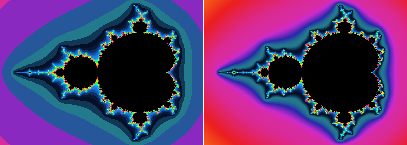
Coloring by the raw integer iteration count bands the image into visible rings. DoomFracting uses a continuous fractional count instead (the standard formula, attributed to Linas Vepstas):
Standard double-precision floating point gives roughly 15–17 significant digits. DoomFracting caps zoom at \(5\times10^{15}\times\) to stay just short of where individual pixels stop being distinguishable — Part VII covers how dedicated deep-zoom software routes around this entirely.
Distance estimation (DEM)
Knowing how close a pixel is to the boundary — not just how it's colored — is what enables a crisp anti-aliased edge, or a lighting model that treats the boundary as a cliff. The Hubbard–Douady distance estimate answers this via the map's own derivative:
Where DoomFracting's Julia renderer stands today: the shared orbit routine always computes \(\partial z_n/\partial c\) (the Mandelbrot derivative) — exactly correct for Mandelbrot renders. For Julia, the meaningful derivative would be \(\partial z_n/\partial z_0\) instead, which the engine doesn't yet track. Because Julia's renderer never applies DEM or Glow, this has no visible effect today — but Orbit Traps and 3D Relief have no such dependency at all; they simply aren't offered for Julia yet, a separate scope choice.
The raw distance-to-pixel ratio spans dozens of orders of magnitude, so DoomFracting compares on a \(\log_2\) scale instead of linear:
Beyond escape-time: traps, glow, relief
Orbit traps
Tracks the closest an escaping orbit ever comes to either axis, \(t = \min_k \min(|\mathrm{Re}(z_k)|, |\mathrm{Im}(z_k)|)\), and paints a bright vein where it passed close: \(\text{vein} = \operatorname{clamp}(t/0.4)^{0.45}\), blended against a 0.35 brightness floor so a trapped pixel never goes fully dark.
Glow
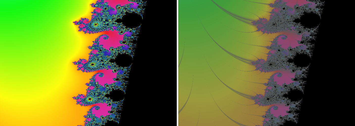
An additive neon halo, purely a function of the DEM distance, decaying exponentially in units of pixel footprint — only pixels genuinely near the boundary light up. In SOUND mode, live microphone treble energy boosts its intensity in real time.
3D relief (Blinn–Phong shading)
Treats the smooth iteration count as a height field, \(H = \ln(1+\nu)/\ln(1+\text{maxIter})\), takes a central-difference surface normal from its gradient, and lights it with a standard diffuse + specular model — a genuine 3D lighting model aimed at a mathematically synthetic surface.
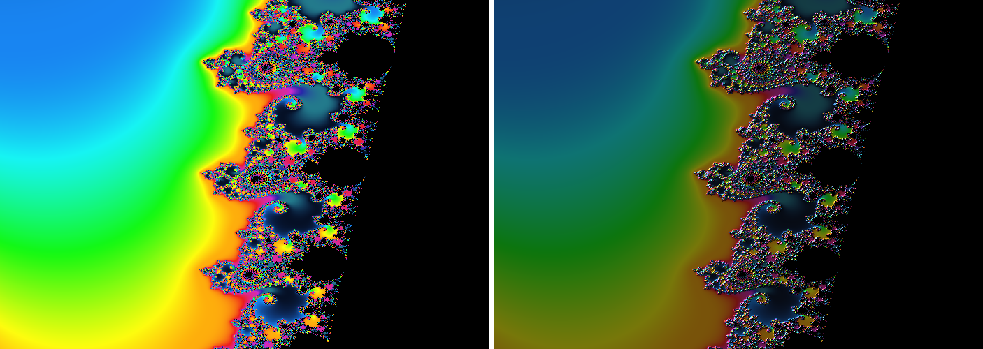
Palette generation and animation
DoomFracting's default ("Fractint-style") generator scatters 3–6 random HSV control points (saturation and value both ≥ 0.7, for vivid color) around a loop, resampled to 256 entries with cosine easing and shortest-path hue interpolation, so the table cycles seamlessly.
In SOUND mode, vocal pitch (80–1,000 Hz, mapped logarithmically) rotates the whole color wheel, and overall volume displaces the palette forward by up to 0.12 of a cycle — a fast attack, gentle release, heartbeat-like pulse rather than continuous rotation.
AUTO: automated boundary exploration
- Candidate scoring. Every exterior pixel within the central 70% of the viewport is scored by its DEM distance.
- Candidate pool. The 40 closest-to-boundary points are kept; flatter, boundary-distant regions are discarded.
- Randomized pick and zoom. AUTO picks uniformly at random among those 40, then zooms by a randomized factor between 1.4× and 2.2×.
- Cadence. A 7.0-second timer starts only after each render finishes.
- Undo and reset. Fully undoable via the ordinary swipe-back gesture; past \(10^{15}\times\) zoom, AUTO resets to the initial view and starts a fresh path.
Recent advances (beyond what DoomFracting implements)
Double-precision arithmetic loses meaningful precision once the zoomed region shrinks below about \(10^{-15}\)–\(10^{-16}\) in width. Perturbation theory, popularized by K. I. Martin's SuperFractalThing (2013), sidesteps this: compute one reference orbit at arbitrary precision, then iterate only the low-precision difference from it for every other pixel — a quantity that doesn't lose meaningful information, because the high-precision digits cancel out.
Claude Heiland-Allen's Kalles Fraktaler 2+ extended this with series approximation, skipping large blocks of early iterations outright — roughly another 10× on top of perturbation alone. A 2010 zoom animation reached \(2.1\times10^{275}\times\) magnification the hard way (12 CPU cores, six months); modern perturbation-and-series renderers reach comparable and far greater depths in minutes, on consumer hardware.
DoomFracting's own \(5\times10^{15}\times\) ceiling is exactly the double-precision wall this technique exists to route around — the single most impactful "how would you actually go deeper" answer available, and a genuine architecture change rather than a tuning tweak.
Fascinating properties
- The Mandelbrot set is connected — proved by Douady and Hubbard in 1982, overturning Mandelbrot's own early suspicion that it might be scattered dust.
- Whether it's locally connected (MLC) is still open — one of complex dynamics' central unsolved problems. Large classes of parameters are proven (Yoccoz, Lyubich, Kahn); a full proof would imply hyperbolic dynamics is dense among quadratic polynomials.
- The boundary has Hausdorff dimension exactly 2 — proved by Shishikura in 1998, despite (by connectedness) enclosing zero area.
- "Baby Mandelbrot" copies are never exactly self-similar — only asymptotically so — except at Misiurewicz points, where the structure is genuinely exact under repeated zooming.
- Cardioid bulbs are indexed by rational numbers, laid out exactly like the Stern–Brocot / Farey tree: the bulb at angle p/q has period q and q−1 antennae.
- The real-axis slice is the period-doubling bifurcation diagram, shrinking toward the Feigenbaum constant \(\delta \approx 4.6692016\ldots\) — the same constant governing period-doubling chaos in unrelated real-world systems.